When data scientists or analysts outside the software development team analyze the data for insights, many use R for statistical summaries and publication-quality visualizations of the data. But first, to get to the data from the shared data store, those users, many of whom have limited background in SQL and data connectivity, first need to get to the data from the shared data store.
Getting to data is complicated (sort of)
The R language does not include built-in relational database access capability, but there are many data access interfaces available from the various RDBMS vendors and open source implementations. Unfortunately, setting up a connection requires an understanding of the network, server, and database and using each of the built-in access capabilities requires learning the syntax for that vendor. Furthermore, configuration requires testing using an actual username with database privileges.
For the data scientist/analyst in the organization, networking and configuring ODBC falls under IT functions. Sometimes this makes it difficult (depending on your company) to even get started in accessing server-side relational data sources. If you don’t have an IT department, you’ll have to make sure you have permissions to install the correct driver on the server and/or the client, as well. With the many RDBMS implementations, you will be writing code that is either platform-specific or requires relatively complex, platform-specific installation steps.
Data scientist and data analysts consider packages such RJDBC, RODBC and other. To add to the complexity, RJDBC uses a combination of a JDBC compliant database driver and Java Runtime Environment (JRE) to exchange data between R and the database server.
Here are some of the items the hapless data scientist needs for configuring the database listener:
- Hostname or IP
- Port, e.g., 1521
- Service name or SID, e.g., ORCL
- Username
- Password
In addition, you may have install the R package and load the library for the low-level interface to Java VM – rJava.
An alternative to RJDBC is RODBC. Again, connecting to a database from the RODBC driver involves identifying the location of the server, the name of the database, and supporting credentials. Using the RODBC path will force the data scientist to learn and use R functions such as sqlFetch() to retrieve the data into R. Any valid SQL query can be sent to the database server using the sqlQuery() function. If you have the authority to DROP tables or remove data, then you can use the the sqlDrop() or sqlClear() functions. Obviously, there is a bit of a learning curve for each of these package functions. But first, you will have to code the database connection for the database vendor.
Some examples:
Connecting to Oracle using RODBC
library(RODBC)
channel <- odbcConnect("someDSN", uid="root", pwd="password")
dataFrame <- sqlQuery(channel, "SELECT * FROM dbname.myTable");
close(channel);
Connecting to MS SQL Server using RODBC
library(RODBC)
channel <- odbcDriverConnect('driver={SQL Server};server=MSqlsrvhost;database=mydbname;trusted_connection=true')
dataFrame <- sqlQuery(channel, 'select * from information_schema.tables')
Note that in the above connection string function, more flexibility is available via the function, odbcDriverConnect. Syntax can be described as “DSN=dsn;UID=uid;PWD=pwd” . Or the function can be constructed without a DSN if you specify a driver as in the example above — DRIVER=, as well as other driver-specific parameters that you can include. Definitely not a fun way to start off the process of just getting a data frame in place to do your exploratory data analysis and not what you were hired to do.
Connecting to MySQL can have you using another method, the RMySQL package.
install.packages("RMySQL")
library(RMySQL)
Once the RMySQL library is installed, you’ll have to create a database connection object:
myconn <- dbConnect(MySQL(), user='user', password='password', mydbname='database_name', host='urlForHost')
dbListTables(myconn)
… will list the base tables for the database (mydbname) user in the dbConnect function
You can now enter your SQL command via:
dataFrame <-dbGetQuery(myconn,'select * from mytable')
You’ll also want to consider housekeeping chores such as a disconnect using:
dbDisconnect(myconn)
All the moving parts of ODBC
You should note that an ODBC environment consists of an ODBC Driver Manager and an ODBC compliant driver for the database server you would like to use.
On Windows, the ODBC Driver Manager is built into the platform, but on Linux or other platforms an ODBC Driver Manager will probably have to be installed. ODBC driver managers such as unixODBC and iODBC will be needed (not to mention iODBC is used by macOS). The connection to the particular RDBMS needs an ODBC driver. These may come with the RDBMS or the ODBC driver manager or be provided separately by the RDBMS vendor. This means that for some RDBMSs there are several different ODBC drivers available, and they can behave differently if and when you need to switch around from one backend data store to another.
The easy way
An alternative to the connectivity considerations seen above can be realized by the SlashDB data API gateway which serves as a web service API. If that sounds foreign, fear not. It all begins with a friendly web-based GUI.
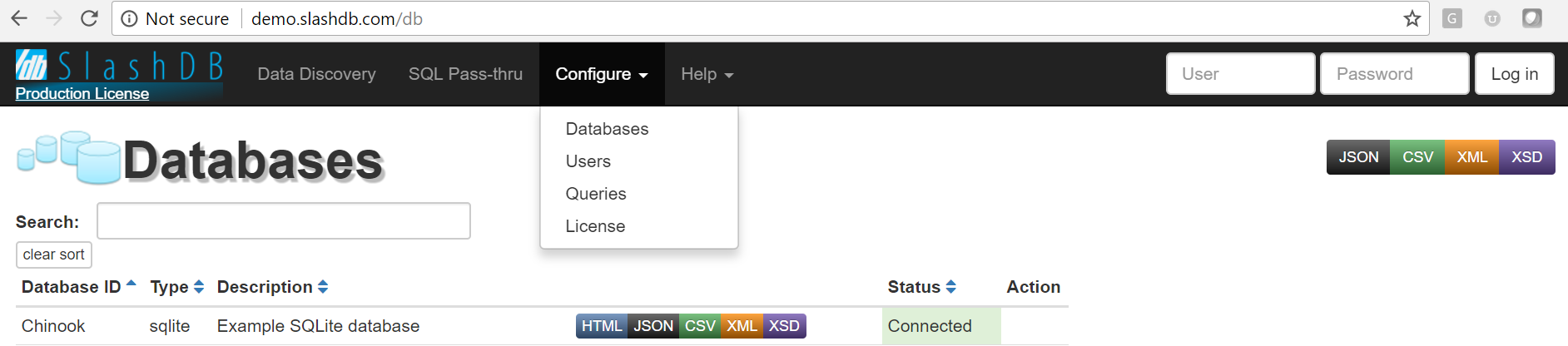
Once SlashDB is installed and connected to your databases, using an intuitive user interface (above), authorized users and their apps can instantly reach your data via reference to URLs. This allows the data scientist/analyst to concentrate on what they do best. Using the Data Discovery feature data analysts browse through available data tables, filter down and even traverse to related records.
SlashDB is unique in that as you browse through data tables in HTML, the URL from the browser’s address bar will be the same for the API, only for a different data format (i.e. JSON, CSV, XML).
The following URL points to an individual record from the Employee table in the Chinook database in HTML format. You can look at it.
Corresponding API endpoints in JSON, CSV and XML for programs to consume are simply:
- https://demo.slashdb.com/db/Chinook/Employee/EmployeeId/1.json
- https://demo.slashdb.com/db/Chinook/Employee/EmployeeId/1.csv
- https://demo.slashdb.com/db/Chinook/Employee/EmployeeId/1.xml
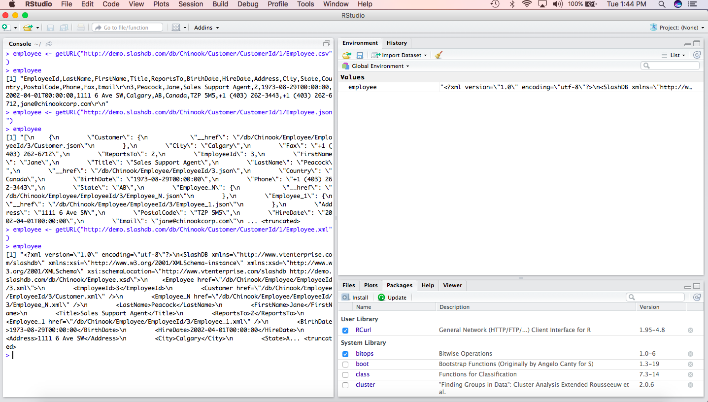
Example in R
Here is the above example of a SlashDB HTTP Restful Web Service integration into R.
Or fetch the whole table formatted as CSV straight into a data.frame, in just one line of code:
> read.csv('http://demo.slashdb.com/db/Chinook/Employee.csv')
  EmployeeId LastName FirstName               Title ReportsTo           BirthDate            HireDate                     Address       City State Country PostalCode             Phone               Fax                    Email
1          1    Adams    Andrew     General Manager        NA 1962-02-18T00:00:00 2002-08-14T00:00:00         11120 Jasper Ave NW   Edmonton    AB  Canada    T5K 2N1 +1 (780) 428-9482 +1 (780) 428-3457   andrew@chinookcorp.com
2          2  Edwards     Nancy       Sales Manager         1 1958-12-08T00:00:00 2002-05-01T00:00:00                825 8 Ave SW    Calgary    AB  Canada    T2P 2T3 +1 (403) 262-3443 +1 (403) 262-3322    nancy@chinookcorp.com
3          3  Peacock      Jane Sales Support Agent         2 1973-08-29T00:00:00 2002-04-01T00:00:00               1111 6 Ave SW    Calgary    AB  Canada    T2P 5M5 +1 (403) 262-3443 +1 (403) 262-6712     jane@chinookcorp.com
4          4     Park  Margaret Sales Support Agent         2 1947-09-19T00:00:00 2003-05-03T00:00:00            683 10 Street SW    Calgary    AB  Canada    T2P 5G3 +1 (403) 263-4423 +1 (403) 263-4289 margaret@chinookcorp.com
5          5  Johnson     Steve Sales Support Agent         2 1965-03-03T00:00:00 2003-10-17T00:00:00                7727B 41 Ave    Calgary    AB  Canada    T3B 1Y7  1 (780) 836-9987  1 (780) 836-9543    steve@chinookcorp.com
6          6 Mitchell   Michael          IT Manager         1 1973-07-01T00:00:00 2003-10-17T00:00:00        5827 Bowness Road NW    Calgary    AB  Canada    T3B 0C5 +1 (403) 246-9887 +1 (403) 246-9899  michael@chinookcorp.com
7          7     King    Robert            IT Staff         6 1970-05-29T00:00:00 2004-01-02T00:00:00 590 Columbia Boulevard West Lethbridge    AB  Canada    T1K 5N8 +1 (403) 456-9986 +1 (403) 456-8485   robert@chinookcorp.com
8          8 Callahan     Laura            IT Staff         6 1968-01-09T00:00:00 2004-03-04T00:00:00                 923 7 ST NW Lethbridge    AB  Canada    T1H 1Y8 +1 (403) 467-3351 +1 (403) 467-8772    laura@chinookcorp.com
As seen above, using SlashDB, you can decide whether you want the output to be returned in either JSON, XML, or CSV format. You can use tools such as jsonlite and xml2 to allow you to parse the response. These packages will turn HTTP responses into R objects that you can then use in your R scripts and RStudio environment (more below). You can optionally use the tidyverse package features to tidy the data and then transform it to get the data into the shape you want it in for your analysis and data visualization.
Live demo with R-Studio
To see SlashDB in action, we set up an RDBMS a test server environment containing relational data found in the Chinook sample database. Details of this relational database example project can be found at https://github.com/lerocha/chinook-database . The Chinook data model represents a digital media store (e.g. iTunes), including tables for artists, media tracks, invoices, customers and more.
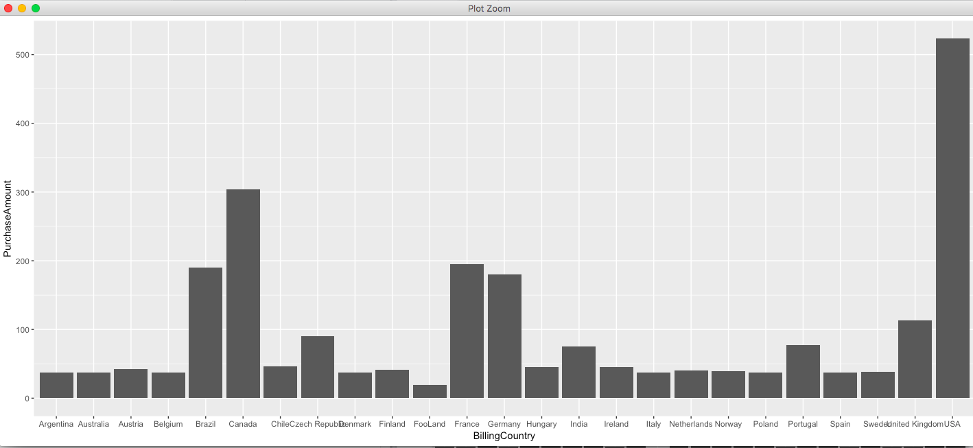
In this R example, we first load up the libraries needed for retrieving and parsing the output of the relational data returned in the HTTP response. The SlashDB endpoint we’ll use is: http://demo.slashdb.com/db/Chinook/Invoice.json which enumerates 400+ purchases found within the Invoice base table in the Chinook database. The full script is presented here:
#  Example using SlashDB: Plot the total purchases from the media store by country
library(httr)
library(jsonlite)
library(magrittr)
library(ggplot2)

ChinookInvoices <- GET("http://demo.slashdb.com/db/Chinook/Invoice.json")

ChinookInvoices$status_code
ChinookInvoices$headers$'content-type'
names(ChinookInvoices)
# Get the content of the HTTP response
text_content <- content(ChinookInvoices, as = 'text', encoding = "UTF-8")

text_content


# parse with jsonlite
json_content <- text_content %>% fromJSON
json_content
BillingCountry <- json_content$BillingCountry
TotalPurchaseAmount <- json_content$Total


dat <- data.frame(
    BillingCountry,
    TotalPurchaseAmount
)

p <- ggplot(data=dat, aes(x=BillingCountry, y=TotalPurchaseAmount)) +
    geom_bar(stat="identity")


p
The bar chart is displayed as:
Summary
Using the connected data sources and single URL references will assure that you never need to extract data and do your analysis from stale CSV files and other client-side extract files. The data connectivity problems inherent in JDBC and ODBC are mitigated and the use of SlashDB’s SQL Pass-thru and data transversal features will allow easy navigation of the relational data — a pleasant alternative to writing and debugging SQL Select statements.